The Perceptron : a learning binary classifier [nn part 2]
In this article I want to introduce historic models that led to the current artificial neurons. I am usually not a big fan of going through the history of a technology just to learn the current one, but in the case of neural networks, it is common to see record-breaking models built from old ideas.
In the previous article we ended up with the following formula :
\[y = \mathcal{H}(\mathbf{x} \cdot \mathbf{w}-b)\]This is almost how Warren McCulloch and Walter Pitts proposed in 1943 a model of a neuron called a Threshold Logic Unit. Their original idea imposes restrictions on the values of x and w, but let’s forget about them.
So yes, a “1943 neuron” is a binary linear classifier.
In the case of neurons, x is called the input(s) (or features), y is the output, w contains the weights, and b is the threshold or bias unit.
We can represent the previous equation with the following computational graph :
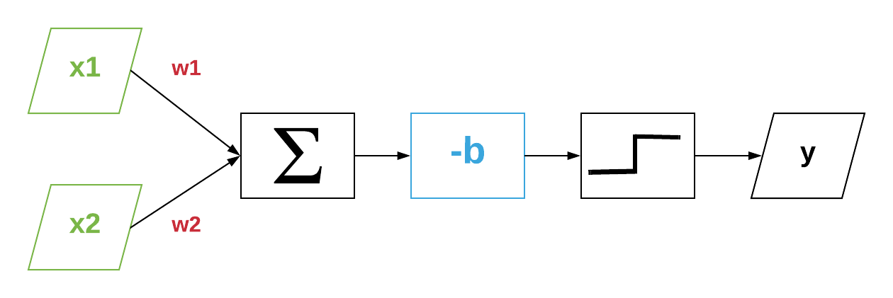
It’s common to use this type of graph to visualize how neurons and neural networks work.
This classifier has two parameters w and b. Finding appropriate values to them manually is pretty straightforward in up to 3-dimensional spaces. But it gets harder when we want to have more features, and we don’t want to do the hard work.
We can learn the values of w and b using a perceptron.
The percetron was first referenced in 1957 by Frank Rosenblatt. Rosenblatt focused his attention on the feasibility of constructing a device possessing perception and recognition abilities.
To quote Rosenblatt himself (1962) :
A perceptron is first and foremost a brain model, not an invention for pattern recognition… its utility is in enabling us to determine the physical conditions for the emergence of various psychological properties.
The meaning of a perceptron can be confusing because it has evolved through the years, however we could define a perceptron as an algorithm for learning the values of the parameters of binary classifiers.
Learning is all about making mistakes and correcting them to get better, right ?! Well that is how perceptrons work. Perceptrons learn by examples.
To be able to find w and b, we first initialize them to random values. Then, we try the model with these values and get predictions :
\[\hat{y}\]We compare it to the reality (y), and we finally update the parameters. We repeat these operations until we find correct values.
The process of comparing the reality (y) and the predictions (y hat) computed by the model is called “supervised learning”.
The perceptron is an old model and my goal is not to present how it works, but to introduce ideas that will help us understand how/why neural networks work.
Random notes
I am not satisfied by this article, but I want to move on to help me think about how to organize my ideas. This serie was a mistake haha.
sources :
- https://blogs.umass.edu/brain-wars/files/2016/03/rosenblatt-1957.pdf
- https://www.cs.cmu.edu/afs/cs.cmu.edu/academic/class/15381-f01/www/handouts/110601.pdf
- http://www.cs.princeton.edu/~tcm3/docs/mapl_2017.pdf
- http://www2.fiit.stuba.sk/~kvasnicka/Logika/Lecture08/Kvasnicka_Pospichal_SETINAIR%202013.pdf
A perceptron is a system able to learn to recognize similarities or identities between patterns of optical, electrical or tonal information, in a manner which may be closely analogous to the perceptual processes of a biological brain. The proposed system depends on probabilistic rather than deterministic principles for its operation, and gains its reliability from the properties of statistical measurements obtained from large populations of elements. A system which operates according to these principles will be called a perceptron.