Understand how binary linear classifiers work [Neural network part 1]

This article is the first of a serie about neural networks. This article gives the mathematical intuiton behind the most basic classifiers there are : binary and linear classifiers. The knowledge aquired in this article will help us understand what a neuron is, and how it works.

A classifier is binary when it classifies data into one of 2 possible classes :

• 0 or negative samples
• 1 or positive samples

A classifier is linear when the samples are linearly seperable. It means that you can separate the positive and negative samples by a line.

Let’s say we have positive and negative examples, and we want to classify them.

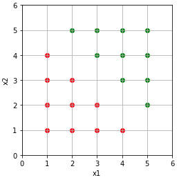
Each sample has two features x1 and x2, let’s note y the class of the sample, such as :

\(y \in \left \{ 0,1 \right \}\) The red samples will be the negative ones, and the green ones will be the positive.

To classify them, the obvious thing to do is to seperate them by a line :

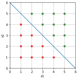
Ok, nice, but how do we actually know that an example is a positive or a negative one ?

Weeeeellll, using maths !

Let’s say we have positive and negative examples seperate by the blue line of equation : \(x2 = -x1 + 6\). Note that this line has a direction vector :

\[\mathbf{d} = \begin{pmatrix}1\\-1\end{pmatrix}\]

From this vector we can easily find a normal vector (red vector) :

\[\mathbf{u} = \begin{pmatrix}1\\1\end{pmatrix}\]

To make our life easier, we transform this vector into a unit vector :

\[\mathbf{w} = \frac{\mathbf{u}}{\|\mathbf{u}\|}\] \[\|\mathbf{w}\| = 1\]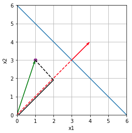

We want to classify the purple sample. This sample can be represented by the green vector :

\[\mathbf{x} = \begin{pmatrix}x1\\x2\end{pmatrix}\]

To classify this sample, the idea is to project \(\mathbf{x}\) (the green vector) on \(\mathbf{w}\) (equivalent to the red vector) to obtain the solid black segment of length \(l\) :

\[l = \|\mathbf{x}\| \cdot \cos(\mathbf{w},\mathbf{x})\]

From the dot product definition we know that :

\[\mathbf{w} \cdot \mathbf{x} = \|\mathbf{w}\| \cdot \|\mathbf{x}\| \cdot \cos(\mathbf{w},\mathbf{x}) = \|\mathbf{w}\| \cdot l\]

We can rewrite \(l\) as :

\[l = \frac{\mathbf{w} \cdot \mathbf{x}}{\| \mathbf{w} \|}\]

Because \(\mathbf{w}\) is a unit vector, we can finally write :

\[l = \mathbf{w} \cdot \mathbf{x}\]

To determine if an example is positive or negative, we just need to look if it’s bellow or above the line. So we just need to compare \(l\) to the length of the red dashed line (\(b\)).

\[\begin{cases} 1 & \text{ if } l\geq b \\ 0 & \text{ if } l < b \end{cases}\]

or

\[\begin{cases} 1 & \text{ if } l-b\geq0 \\ 0 & \text{ if } l-b < 0 \end{cases}\]

To write this down in a single equation, we can use the “Heaviside step function” defined by :

\[\mathcal{H}(t) = \begin{cases} 1 & \text{ if } t \geq 0 \\ 0 & \text{ if } t < 0 \end{cases}\]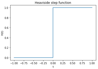

If we replace \(t\) by \(l-b\) we obtain:

\[y = \mathcal{H}(l-b)\]

and with the complete formula:

\[y = \mathcal{H}(\mathbf{x} \cdot \mathbf{w}-b)\]

And there we go, we have a linear binary classifier.